Signals with Small Perturbations

Voice signals exist along a continuum from perfectly periodic (theoretical) to completely aperiodic (aphonic). Type 1 signals occupy the region closest to perfect periodicity—they consist of nearly periodic waveforms with small, random cycle-to-cycle variations. These signals characterize normal or near-normal phonation and represent the domain where traditional perturbation analysis remains valid and meaningful. Understanding Type 1 signals requires examining their acoustic characteristics, the measurement methods applied to them, the assumptions underlying these methods, and the boundaries beyond which conventional analysis breaks down.

Defining Type 1 Signals

Type 1 signals represent voice production where the fundamental oscillatory mechanism operates stably and predictably, with only minor deviations from pure periodicity. These signals possess identifiable individual cycles with consistent fundamental frequency and amplitude, allowing reliable period-to-period tracking.

Acoustic Characteristics

Type 1 signals exhibit several defining features:

Nearly periodic waveform: Each glottal cycle produces a recognizable pulse with similar shape to adjacent cycles. The fundamental period varies slightly from cycle to cycle, but remains clearly identifiable.

Small perturbations: Cycle-to-cycle variations in period (jitter) typically remain below 1-2% in healthy voices. Amplitude variations (shimmer) similarly stay within 3-5% ranges. These small perturbations represent biological noise rather than fundamental instability.

High harmonics-to-noise ratio (HNR): The periodic component dominates the signal, with noise constituting a minor fraction of total acoustic energy. HNR values typically exceed 10-15 dB in Type 1 signals.

Stable spectral structure: Harmonic peaks appear at integer multiples of the fundamental frequency with minimal spectral noise between harmonics. Formant structure remains evident and stable.

Identifiable fundamental frequency: Pitch tracking algorithms can reliably extract F₀ across the signal duration without ambiguity or tracking errors.

Physiological Correlates

Type 1 signals reflect stable phonatory biomechanics:

• Consistent vocal fold oscillation with regular mucosal wave propagation
• Adequate and relatively symmetrical glottal closure
• Stable subglottal pressure and airflow
• Effective neuromuscular control with minimal tremor or spasm
• Appropriate vocal fold tension and stiffness balance

These physiological conditions characterize normal voice production and mild voice disorders that preserve basic oscillatory stability while introducing small perturbations.

Valid Measurement Domain

Type 1 signal classification proves critical because conventional perturbation measures—jitter, shimmer, and related indices—assume nearly periodic signals. Applying these measures to strongly aperiodic signals (Type 2 or Type 3) produces misleading or meaningless results.

Assumptions of Perturbation Analysis

Traditional jitter and shimmer calculations rest on several fundamental assumptions:

Cycle identification: The signal contains discrete, identifiable cycles with one fundamental period each. Period detection algorithms can reliably mark cycle boundaries.

Small deviations from periodicity: Variations represent minor fluctuations around a stable mean period and amplitude. The perturbations constitute “noise” added to an underlying periodic signal rather than fundamental signal instability.

Random or pseudo-random perturbations: Cycle-to-cycle variations lack systematic structure at frequencies different from the fundamental. Any modulation components remain much smaller than the basic period.

Stationary statistics: The mean period and amplitude remain relatively constant throughout the analysis window. Short-term trends and drifts stay minimal.

Single fundamental frequency: The signal contains one dominant F₀, not multiple competing frequencies (as in diplophonia or subharmonic generation).

When these assumptions hold—which defines Type 1 signals—perturbation measures provide meaningful acoustic indices correlating with vocal function and perceived voice quality.

Breakdown Beyond Type 1

When signals violate these assumptions, perturbation measures become problematic:

Strong tremor or vibrato (Type 2): The systematic modulation at 4-8 Hz appears as elevated “jitter” and “shimmer,” but these reflect intentional or pathological oscillation rather than random cycle-to-cycle variability. Computing conventional perturbation values conflates distinct phenomena.

Subharmonics and diplophonia (Type 2): Multiple competing frequencies confuse period detection. Algorithms may lock onto one component, alternate between components, or fail entirely. Resulting “jitter” values reflect algorithm confusion rather than true perturbation.

Chaotic signals (Type 3): The fundamentally aperiodic nature means period detection becomes arbitrary. While algorithms produce numerical results, these lack meaningful interpretation.

This measurement validity restriction makes signal typing—distinguishing Type 1 from Type 2 and Type 3—essential before applying perturbation analysis.

Period Detection Algorithms

All perturbation measures depend critically on accurate identification of the fundamental period for each cycle. Various algorithms approach this challenge differently, with implications for measurement accuracy and reliability.

Waveform Peak Picking

The simplest approach identifies peaks in the acoustic waveform, treating the interval between peaks as one period. This method works reasonably well for high-quality Type 1 signals but faces several limitations:

Harmonic interference: Multiple harmonics create multiple peaks per cycle, potentially confusing peak detection Amplitude variations: Large shimmer may cause some peaks to fall below detection threshold Low signal-to-noise ratio: Background noise can introduce spurious peaks Formant effects: Vocal tract resonances modulate harmonic amplitudes, creating misleading peak patterns

Improvements include bandpass filtering to isolate the fundamental frequency region, though this assumes accurate prior F₀ estimation and can introduce phase distortion affecting timing measurements.

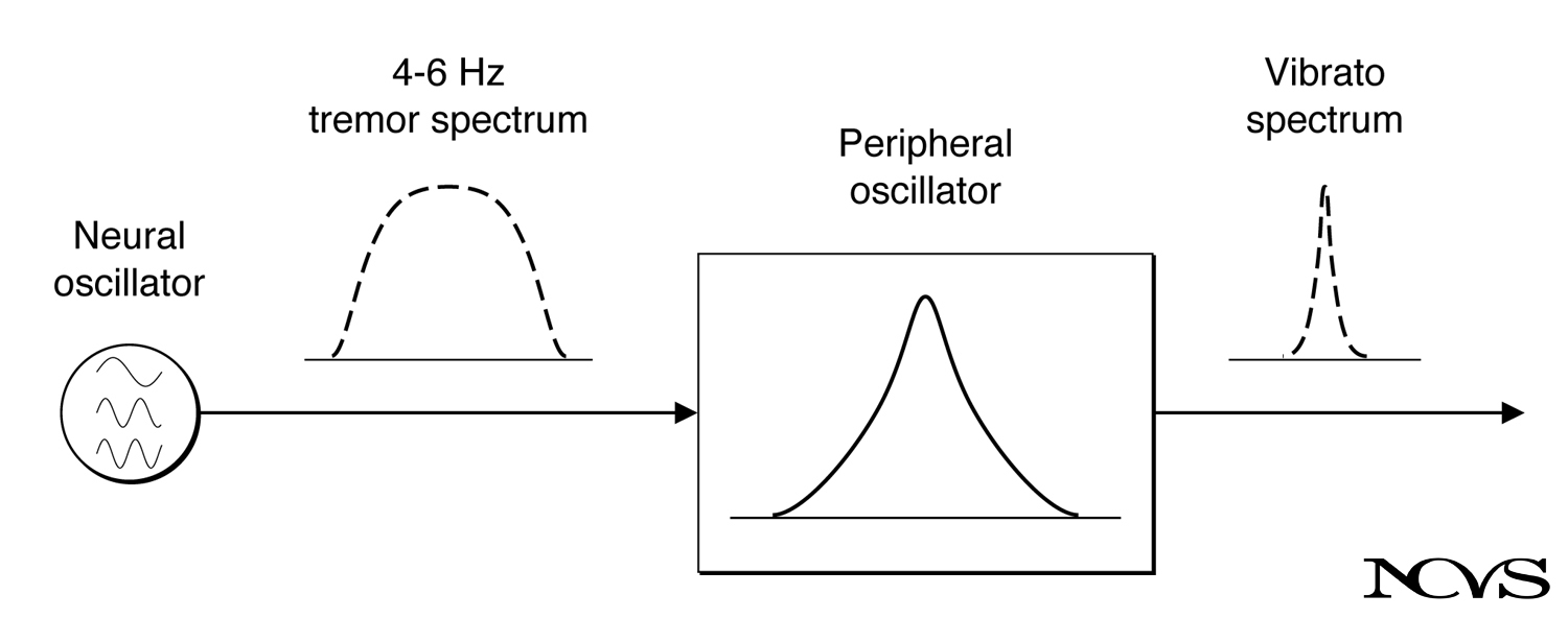Figure 11.7: Comparison of different signal types showing Type 1 signals with small perturbations, Type 2 signals with modulation, and Type 3 signals with aperiodicity. Period detection reliability decreases dramatically as signal type progresses.

Autocorrelation Methods

Autocorrelation computes the correlation between a signal and time-shifted versions of itself. The time lag producing maximum correlation indicates the fundamental period:

R(τ) = Σ x(t) × x(t + τ)

The first major peak in R(τ) (excluding the zero-lag peak) identifies the period. This method proves more robust than peak picking because:

• It uses the entire waveform shape, not just amplitude peaks
• It averages across the analysis window, reducing noise sensitivity
• It inherently seeks periodicity rather than assuming specific peak patterns

Limitations include:

• Requires choice of search range (minimum and maximum plausible F₀)
• Can produce “octave errors” (locking to 2T rather than T)
• Assumes relative stationarity within the analysis window
• Computational cost increases with long analysis windows

Cepstral Analysis

The cepstrum applies inverse Fourier transform to the log power spectrum:

Cepstrum = IFFT[log|FFT[x(t)]|²]

Periodicity in the original signal manifests as peaks in the cepstrum at quefrencies (time-like domain from cepstral analysis) corresponding to the fundamental period. The cepstrum effectively separates excitation (fundamental period) from filter (vocal tract resonances), making it relatively immune to formant effects.

Advantages:

• Robust to spectral tilt and formant effects
• Clear separation of fundamental from harmonic structure
• Well-suited for speech where source-filter independence applies

Disadvantages:

• Requires sufficient signal duration for frequency resolution
• Assumes approximate stationarity during analysis window
• May struggle with very breathy or rough voices where harmonics weaken

Waveform Matching

Waveform matching algorithms correlate template waveforms (individual cycles) with subsequent portions of the signal, identifying the lag producing best match as the period. This approach can track gradual period changes more accurately than fixed-window methods.

The algorithm:

1. Extract a reference cycle from a stable portion of signal
2. Cross-correlate this template with subsequent signal
3. Identify peak correlation lag as period for that cycle
4. Update template for next cycle to track gradual changes

This technique handles moderate jitter better than methods assuming stable period across long windows, though computational cost can be high.

Jitter Measurement Variants

Once periods are identified, multiple algorithms exist for quantifying period perturbation. Different measures capture different aspects of period variability.

Absolute Jitter

Absolute jitter (also called jitter absolute or Jita) computes the average absolute difference between consecutive periods:

Jita = (1/(N-1)) × Σ|Tᵢ₊₁ - Tᵢ|

This produces a value in time units (microseconds or milliseconds). For a voice with 100 Hz mean F₀ (10 ms period) and 50 μs absolute jitter, adjacent cycles differ by 50 μs on average.

Absolute jitter’s advantage lies in its direct interpretability—it quantifies actual timing variations. However, its dependence on the mean period makes cross-speaker comparisons problematic unless speakers have similar F₀.

Jitter Percent

Jitter percent (Jitt%) normalizes absolute jitter by the mean period:

Jitt% = (Jita / T̄) × 100%

This dimensionless percentage enables comparison across speakers and fundamental frequencies. A speaker with 100 Hz F₀ and 50 μs absolute jitter has 0.5% jitter. Another speaker with 200 Hz F₀ (5 ms period) and 25 μs absolute jitter also has 0.5% jitter—their perturbations are equivalent relative to their period.

Jitter percent represents the most commonly reported perturbation measure in clinical contexts, with normal values below 1% and pathological voices often exceeding 1-2%.

Relative Average Perturbation (RAP)

RAP compares each period to the smoothed average of itself and two neighbors:

RAP = (1/(N-2)) × Σ|Tᵢ - (Tᵢ₋₁ + Tᵢ + Tᵢ₊₁)/3| / T̄

The three-period smoothing reduces sensitivity to transient irregularities or measurement noise, providing a more stable estimate. RAP typically yields slightly lower values than jitter percent because the smoothing removes some apparent perturbation.

Clinical research suggests RAP may discriminate between voice types more effectively than simple jitter percent in some pathological conditions, though both measures show considerable overlap between normal and disordered populations.

Period Perturbation Quotient (PPQ)

PPQ extends the smoothing concept to five consecutive periods:

PPQ = (1/(N-4)) × Σ|Tᵢ - (Tᵢ₋₂ + Tᵢ₋₁ + Tᵢ + Tᵢ₊₁ + Tᵢ₊₂)/5| / T̄

This greater smoothing provides even more stability but at the cost of losing information about rapid perturbation variations. PPQ proves particularly useful for voices with occasional large perturbations—the smoothing prevents these outliers from dominating the measure.

Different software packages may implement slightly different windowing or weighting schemes, producing variations in the exact PPQ values despite following the general approach.

Shimmer Measurement Variants

Amplitude perturbation measures parallel period perturbation measures but operate on cycle-to-cycle amplitude variations.

Amplitude Measurement Approaches

Defining “amplitude” for a vocal cycle presents several options:

Peak-to-peak amplitude: The difference between maximum and minimum sample values within a cycle. Simple to compute but sensitive to noise and harmonic interference.

RMS amplitude: Root-mean-square amplitude averaged across the cycle. More stable than peak-to-peak and less sensitive to noise, but requires clear cycle boundary identification.

Peak amplitude: Maximum absolute sample value. Simpler than peak-to-peak but loses information about waveform asymmetry.

Different software packages may use different amplitude definitions, contributing to cross-system measurement variability.

Shimmer in Percent

Shimmer percent computes the average absolute amplitude difference between consecutive cycles normalized by mean amplitude:

Shim% = (1/(N-1)) × Σ|Aᵢ₊₁ - Aᵢ| / Ā × 100%

Normal voices typically show shimmer below 3%, with values above 5% suggesting pathology. Like jitter percent, shimmer provides a normalized measure enabling comparison across intensity levels and speakers.

Shimmer in Decibels

Shimmer in dB expresses amplitude variation in decibel units:

Shim(dB) = (1/(N-1)) × Σ|20×log₁₀(Aᵢ₊₁/Aᵢ)|

The decibel scale relates more closely to auditory perception than linear amplitude, potentially improving correlation with perceived roughness. However, shimmer in dB and shimmer percent do not convert linearly—small perturbations show approximate conversion (Shim(dB) ≈ 0.115 × Shim%), but this relationship breaks down for larger perturbations.

Amplitude Perturbation Quotient (APQ)

APQ applies smoothing to amplitude measurements analogously to PPQ for period:

APQ = (1/(N-10)) × Σ|Aᵢ - (Aᵢ₋₅...Aᵢ₊₅)/11| / Ā

The 11-cycle smoothing window provides substantial stability, making APQ particularly useful for voices with large transient amplitude variations that might represent voice breaks or other irregularities rather than typical shimmer.

Cycle-to-Cycle Tracking Requirements

Reliable perturbation measurement requires accurate tracking through the entire signal. Several factors threaten tracking accuracy in Type 1 signals.

Period Doubling and Halving Errors

Period doubling occurs when the algorithm identifies two consecutive cycles as a single cycle, effectively measuring period 2T instead of T. This typically happens when:

• Alternate cycles have markedly different amplitudes
• Odd and even cycles show slightly different waveform shapes (subharmonic components)
• Detection threshold set inappropriately for signal amplitude

Period halving represents the opposite error—identifying one cycle as two, measuring T/2 instead of T. This may occur when:

• Strong second harmonic creates two peaks per cycle
• Bandwidth filtering insufficient to suppress higher harmonics
• Algorithm sensitivity too high, triggering on minor waveform features

Both errors produce artifactually large “jitter” values that reflect algorithm failure rather than true perturbation. Validation requires examining detected periods to identify implausible outliers.

Tracking Through Voice Breaks

Brief voice breaks—moments where phonation interrupts—pose particular challenges. The algorithm must either:

• Detect and exclude the break region from analysis
• Track through despite the disruption (risking erroneous period assignment)
• Terminate analysis at the break

Different software packages handle breaks differently, affecting measured perturbation values. Severe breaks may disqualify a sample from Type 1 classification entirely.

Onset and Offset Regions

Voice onset and offset involve rapidly changing vocal fold dynamics and aerodynamics. Period and amplitude both show systematic trends (not random perturbations) during these transitions. Standard practice excludes approximately the first and last 0.5-1.0 seconds from analysis, focusing on the stable middle portion where Type 1 characteristics best apply.

Normal Values and Clinical Thresholds

Extensive research has established normative data for perturbation measures in healthy voices, though specific values depend on measurement method, vowel, pitch, intensity, and speaker demographics.

Jitter Normal Ranges

Young healthy adults (ages 20-40):

• Jitter percent: 0.3-0.6% (mean), <1.0% (upper normal limit)
• Absolute jitter: 20-50 μs (varies with F₀)
• RAP: 0.2-0.5%
• PPQ: 0.2-0.4%

Older adults (ages 60+):

• Jitter percent: 0.5-1.0% (mean), <1.5% (upper normal limit)
• Age-related increases reflect tissue changes and neuromotor control degradation

Clinical interpretation:

• 1.0-1.5%: Borderline/mild abnormality
• 1.5-3.0%: Moderate abnormality

• 3.0%: Severe abnormality

These thresholds provide rough guidelines but considerable overlap exists between normal and pathological populations, limiting diagnostic sensitivity and specificity.

Shimmer Normal Ranges

Young healthy adults:

• Shimmer percent: 1.0-2.5% (mean), <3.0% (upper normal limit)
• Shimmer dB: 0.15-0.35 dB
• APQ: 1.5-3.0%

Older adults:

• Shimmer percent: 2.0-3.5% (mean), <4.0% (upper normal limit)
• Age effects on shimmer appear less pronounced than on jitter

Clinical interpretation:

• 3.0-5.0%: Borderline/mild abnormality
• 5.0-8.0%: Moderate abnormality

• 8.0%: Severe abnormality

Shimmer shows greater inter-subject variability than jitter, reflecting greater susceptibility to respiratory and acoustic factors beyond oscillatory stability.

Factors Affecting Normal Values

Multiple variables influence perturbation measures even in healthy Type 1 voices:

Fundamental frequency: Jitter increases at very low (<80 Hz) and very high (>300 Hz) F₀ Intensity: Soft phonation increases perturbation; very loud phonation may increase or decrease perturbation Vowel: Different vowels show different stability, with /a/ typically most stable Phonation duration: Perturbation may increase with sustained phonation duration due to fatigue Time of day: Some evidence suggests perturbation varies across the day, possibly reflecting hydration or fatigue Vocal training: Trained singers typically show lower perturbation than untrained speakers

Normative comparisons should ideally match these factors, though clinical practice often uses general population norms.

Harmonics-to-Noise Ratio

While jitter and shimmer quantify periodic component variability, harmonics-to-noise ratio (HNR) assesses the relative strength of periodic versus aperiodic signal components.

Computation Methods

HNR computation involves separating the signal into periodic and aperiodic components:

Comb-filtering approach: The signal spectrum is filtered to retain only harmonic frequency regions (integer multiples of F₀), with the filtered and residual energy compared:

HNR(dB) = 10×log₁₀(E_harmonics / E_noise)

Autocorrelation approach: The autocorrelation function at period lag indicates the signal’s periodicity. High autocorrelation at period T suggests strong periodicity:

HNR(dB) = 10×log₁₀(R(T) / [R(0) - R(T)])

where R(T) is autocorrelation at the fundamental period lag.

Interpretation and Normal Values

Type 1 signals typically show HNR >10-15 dB, indicating the periodic component exceeds noise by this margin. Higher values (>20 dB) characterize particularly stable phonation.

Normal ranges:

• Modal register, normal voices: 15-25 dB
• Mildly impaired: 10-15 dB
• Moderately impaired: 5-10 dB
• Severely impaired: <5 dB

HNR correlates moderately with perceptual breathiness (r ≈ -0.6 to -0.7) and overall voice quality. Low HNR suggests excessive noise from incomplete glottal closure, turbulent airflow, or irregular oscillation.

Relationship to Perturbation Measures

HNR, jitter, and shimmer assess related but distinct aspects of voice quality:

• Jitter/shimmer: Quantify cycle-to-cycle variability in the periodic component
• HNR: Quantifies the strength of the periodic component relative to noise

A voice can have low jitter but also low HNR (stable oscillation with poor closure producing noise). Conversely, high jitter typically accompanies low HNR as irregular oscillation tends to increase noise. Combined assessment provides more comprehensive voice quality characterization than any single measure.

Signal Quality Requirements

Valid Type 1 analysis requires high-quality recordings meeting specific technical standards.

Recording Parameters

Sampling rate: Minimum 20 kHz, preferably 44.1 or 48 kHz. Nyquist theorem requires sampling rate >2× the highest frequency of interest. For accurate perturbation measurement of F₀ up to 500 Hz with harmonics to 4-5 kHz, 20 kHz minimum suffices, though higher rates provide margin.

Bit depth: 16-bit minimum, 24-bit preferred. Higher bit depth improves dynamic range and reduces quantization noise, particularly important for amplitude perturbation measurement.

Microphone: Quality condenser microphone with flat frequency response 80 Hz-10 kHz. Directional (cardioid) pattern reduces ambient noise. Headset microphones provide consistent mouth-to-microphone distance but may introduce low-frequency noise from breath turbulence.

Mouth-to-microphone distance: 10 cm (4 inches) standard. Closer distance increases breath noise; greater distance reduces signal strength relative to ambient noise.

Environment: Quiet room with ambient noise <50 dB SPL. Hard surfaces should be minimized to reduce reverberation, though some acoustic treatment may be impractical in clinical settings.

Signal Processing Considerations

High-pass filtering: Apply high-pass filter at 50-80 Hz to remove low-frequency environmental noise, 60 Hz electrical hum, and microphone handling noise. This filtering typically improves rather than degrades perturbation measurement.

Low-pass filtering: Apply anti-aliasing filter at sampling rate/2. Most analog-to-digital converters include this automatically, but verify to prevent aliasing artifacts.

Avoid compression: Dynamic range compression or normalization after recording can alter amplitude relationships, affecting shimmer measurement. Record at appropriate gain levels initially rather than applying post-recording amplitude changes.

Avoid pitch correction: Some recording software includes automatic pitch correction or “auto-tune” features. These must be disabled as they directly alter the perturbation being measured.

Limitations and Cautions

Despite widespread clinical use, Type 1 signal perturbation analysis faces important limitations.

Measurement Reliability

Test-retest reliability of perturbation measures shows moderate correlation (r ≈ 0.7-0.85) in well-controlled conditions but can decrease substantially with:

• Different recording equipment
• Different analysis software/algorithms
• Different vowel or pitch selections
• Different phonation attempts by the same speaker

This variability limits the utility of perturbation measures for detecting small changes in individual patients over time.

Diagnostic Sensitivity and Specificity

Perturbation measures show considerable overlap between normal and pathological populations. Sensitivity (correctly identifying disorders) and specificity (correctly identifying normals) typically range 70-80%, limiting diagnostic utility when used alone. False negatives occur frequently—many individuals with diagnosed voice disorders fall within normal perturbation ranges.

This limitation reflects multiple factors:

• Voice disorders involve multiple dimensions beyond oscillatory stability
• Compensatory behaviors may maintain near-normal perturbation despite underlying pathology
• Measurement variability creates diagnostic uncertainty near threshold values
• Perceptual impairment can occur without measurable acoustic deviation

Perturbation analysis provides valuable information within comprehensive voice assessment but should not serve as sole diagnostic criterion.

Software and Algorithm Variability

Different acoustic analysis programs implement different algorithms for period detection, cycle marking, and perturbation computation. Studies comparing programs report moderate correlations (r ≈ 0.7-0.9) but systematic differences in absolute values. A voice showing 0.8% jitter in one program might show 1.1% in another—potentially crossing clinical threshold despite analyzing identical recordings.

This variability demands caution when comparing values across studies, clinical sites, or time points where analysis methods changed. Within-system comparisons remain more reliable than across-system comparisons.

Summary

Type 1 signals represent nearly periodic voice production with small random perturbations, characterized by identifiable cycles, stable fundamental frequency, high harmonics-to-noise ratio, and regular spectral structure. These signals define the valid domain for conventional perturbation analysis—jitter, shimmer, and related measures assume near-periodicity and produce meaningful results only when this assumption holds.

Period detection algorithms including peak picking, autocorrelation, cepstral analysis, and waveform matching enable cycle identification, with each method offering distinct advantages and limitations. Multiple jitter variants (absolute, percent, RAP, PPQ) and shimmer variants (percent, dB, APQ) quantify different aspects of cycle-to-cycle variability. Normal values typically show jitter <1% and shimmer <3%, with age, F₀, intensity, and other factors influencing these ranges.

High-quality recordings meeting specific technical standards prove essential for valid measurement. Software and algorithm variability, modest test-retest reliability, and moderate diagnostic sensitivity limit perturbation analysis utility when used alone. These measures provide valuable objective information within comprehensive voice assessment but require interpretation alongside perceptual evaluation, case history, and visualization. Understanding Type 1 signal characteristics and measurement requirements enables appropriate application and interpretation of perturbation analysis in clinical and research contexts.

Key Takeaways

• ✅ Type 1 signals feature nearly periodic waveforms with small perturbations, defining the valid domain for conventional jitter and shimmer analysis
• ✅ Perturbation measures assume identifiable cycles, small deviations from periodicity, and stable statistics—assumptions that break down for Type 2 and Type 3 signals
• ✅ Period detection algorithms including autocorrelation and cepstral methods enable cycle identification with varying robustness to noise and signal degradation
• ✅ Multiple jitter and shimmer variants exist (absolute, percent, RAP, PPQ, APQ), each capturing different aspects of perturbation
• ✅ Normal jitter typically remains below 1%, shimmer below 3%, with age-related increases and clinical thresholds around 1.5% and 5% respectively
• ✅ High-quality recordings (≥20 kHz sampling, 16+ bit depth, quiet environment, proper microphone placement) prove essential for valid measurement
• ✅ Harmonics-to-noise ratio (HNR) assesses periodic versus aperiodic signal components, complementing perturbation measures
• ✅ Measurement reliability and diagnostic sensitivity/specificity limitations require perturbation analysis within comprehensive voice assessment rather than as sole diagnostic criterion

Related Topics

• Jitter and Shimmer
• Perturbations and Fluctuations
• Nonstationarity and Trends
• Bifurcations and Chaos

Further Reading

1. Titze, I. R., Horii, Y., & Scherer, R. C. (1987). Some technical considerations in voice perturbation measurements. Journal of Speech and Hearing Research, 30(2), 252-260.
2. Pinto, N. B., & Titze, I. R. (1990). Unification of perturbation measures in speech signals. Journal of the Acoustical Society of America, 87(3), 1278-1289.
3. Deliyski, D. D., Shaw, H. S., & Evans, M. K. (2005). Adverse effects of environmental noise on acoustic voice quality measurements. Journal of Voice, 19(1), 15-28.
4. Titze, I. R. (1995). Workshop on acoustic voice analysis: Summary statement. Denver, CO: National Center for Voice and Speech.