Variability

Variability in voice production represents a fundamental characteristic of biological systems. Unlike electronic oscillators that can maintain near-perfect stability, the human voice exhibits variation across all time scales—from microsecond differences between successive glottal cycles to hour-to-hour changes in speaking fundamental frequency. Understanding and quantifying this variability provides essential information for distinguishing normal from pathological voice function and for tracking changes during treatment or vocal development.

Time Scales of Variability

Voice variability manifests across multiple temporal domains, each reflecting different underlying physiological mechanisms and requiring distinct measurement approaches. The relevant time scales range from individual glottal cycles to sustained phonation tasks to voice use patterns across days or weeks.

Short-Term Variability

Short-term variability encompasses variations occurring within a single phonatory task, typically measured during sustained vowel production lasting 1-5 seconds. This time scale captures cycle-to-cycle perturbations (jitter and shimmer) as well as any trends or modulations occurring within the analysis window.

For a speaker phonating at 100 Hz, a 3-second analysis window includes approximately 300 glottal cycles. Short-term variability measures quantify how much these cycles differ from one another and from the mean values across the window. This variability arises from neural control noise, respiratory pressure fluctuations, biomechanical irregularities in tissue oscillation, and aerodynamic turbulence—processes operating on millisecond to sub-second time scales.

Medium-Term Variability

Medium-term variability describes changes occurring across multiple phonatory tasks or over several minutes of voice use. A typical protocol might involve repeating a sustained vowel task five times with brief rests between trials. The variability among these trials—differences in mean fundamental frequency, intensity, or perturbation measures—reflects the speaker’s consistency across successive attempts.

This time scale captures effects of motor learning, task familiarity, attention, and early fatigue. Speakers with precise motor control show high consistency across trials, while those with neurological impairment, vocal instability, or poor technique often display greater trial-to-trial variability.

Long-Term Variability

Long-term variability encompasses changes over hours, days, or longer periods. Speaking fundamental frequency, for instance, varies systematically throughout the day, influenced by hydration status, hormonal cycles, cumulative vocal loading, and diurnal rhythms in muscle tension and arousal.

Measuring long-term variability requires sampling voice production across extended periods—for example, recording brief samples at morning, midday, and evening over multiple days. Such protocols reveal baseline voice characteristics, susceptibility to vocal fatigue, and effects of environmental factors or health status changes.

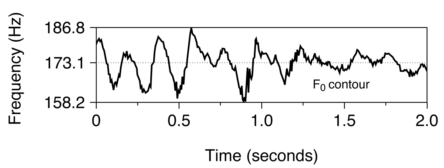Signal analysis across time scales Figure 11.4: Different analysis window lengths reveal variability at different time scales. Short windows capture cycle-to-cycle perturbations, while longer windows show slower modulations and trends.

Statistical Measures of Variability

Quantifying variability requires appropriate statistical measures. The choice of measure depends on the parameter being analyzed, the assumed underlying distribution, and the intended clinical or research application.

Standard Deviation

The standard deviation (SD) represents the most common measure of variability, quantifying the typical deviation of individual values from the mean. For fundamental frequency measured across N glottal cycles:

SD = √[Σ(F₀ᵢ - F₀_mean)² / (N-1)]

Standard deviation has the same units as the measured quantity (Hz for fundamental frequency, dB for intensity), making it interpretable but dependent on the mean value. A 5-Hz standard deviation means something quite different for a soprano singing at 500 Hz versus a bass speaking at 100 Hz.

Coefficient of Variation

The coefficient of variation (CV) normalizes variability relative to the mean, providing a dimensionless measure:

CV = (SD / mean) × 100%

Expressing CV as a percentage enables comparison across different fundamental frequency ranges and different speakers. A CV of 1% indicates that the standard deviation equals 1% of the mean value, whether for a child’s voice at 250 Hz or an adult male at 120 Hz.

The coefficient of variation relates directly to jitter measures, which typically express period variability as a percentage of the mean period. Thus, jitter essentially represents the coefficient of variation for fundamental period.

Range and Percentile-Based Measures

Some applications benefit from measures based on the distribution’s range rather than deviations from the mean. The range (maximum minus minimum) captures the extreme values but proves sensitive to outliers and to the number of cycles analyzed—more cycles increase the probability of extreme values.

Percentile-based measures offer greater robustness. The interquartile range (IQR), spanning the 25th to 75th percentiles, excludes the most extreme values while still capturing central variability. Semi-interquartile range (half the IQR) serves as a robust alternative to standard deviation for non-normal distributions.

Measurement Windows and Stationarity

All variability measures implicitly assume some degree of stationarity—that statistical properties remain constant over the analysis window. This assumption often fails for voice signals, creating methodological challenges.

The Stationarity Assumption

A signal is stationary if its statistical properties (mean, variance, spectral content) do not change with time. Strictly speaking, voice signals are never truly stationary: fundamental frequency drifts, amplitude varies, and voice quality evolves even during sustained phonation attempts.

Nevertheless, voice can be approximately stationary over sufficiently short windows. The art of variability measurement lies in choosing windows short enough to approximate stationarity yet long enough to obtain stable statistical estimates. For typical perturbation measures, 1-3 seconds (100-600 cycles at speech frequencies) represents a practical compromise.

Drift and Trends

Longer analysis windows increasingly reveal systematic trends rather than random variability. A speaker may exhibit decreasing fundamental frequency due to declining subglottal pressure as lung volume decreases. Should this trend be included in variability calculations or removed as a confounding factor?

Standard practice treats trends as distinct from random variability. Removing linear or polynomial trends through detrending algorithms isolates the cycle-to-cycle variations from longer-term systematic changes. However, this separation remains somewhat arbitrary—slow oscillations like tremor occupy an ambiguous zone between trend and variability.

Normal versus Pathological Ranges

Establishing normative data for voice variability enables clinical interpretation of measurements. What constitutes normal variability, and when does variability become clinically significant?

Normal Variability Ranges

Numerous studies have established reference ranges for short-term fundamental frequency and amplitude variability in healthy adults:

Jitter (period variability)

Normal young adults: 0.2-0.6%
Clinical threshold: typically 1.0%
Pathological range: >1.5%

Shimmer (amplitude variability)

Normal young adults: 0.5-2.0%
Clinical threshold: typically 3.0%
Pathological range: >5.0%

These values apply to sustained vowel phonation at comfortable pitch and loudness. Values increase systematically with age, particularly after age 50, reflecting age-related changes in tissue properties, neural control, and respiratory function.

Factors Affecting Normal Ranges

Normal variability depends on multiple factors beyond age:

Phonation Task: Variability typically increases at pitch or loudness extremes compared to comfortable mid-range phonation. Soft phonation often shows greater variability due to reduced glottal closure and lower aerodynamic forces stabilizing oscillation.

Vowel Type: Back vowels like /u/ generally show lower variability than front vowels like /i/, possibly due to differences in laryngeal posturing and vocal tract loading effects on oscillation stability.

Sex: Adult males and females show similar jitter and shimmer values when controlled for fundamental frequency, though females’ higher average F₀ may influence optimal measurement parameters.

Training: Professional voice users (singers, actors) often demonstrate lower variability than untrained speakers, reflecting refined motor control and biomechanical optimization.

Speaking versus Singing Contexts

The functional demand of the task substantially influences variability. Speaking and singing impose different stability requirements and engage different control strategies.

Speech Production

In connected speech, fundamental frequency varies constantly to convey linguistic information (intonation) and emotional content (prosody). What constitutes desirable variability versus problematic instability depends on communicative intent.

For sustained vowels in speech contexts, variability should remain relatively low—indicating stable oscillation and reliable glottal closure. However, in running speech, moment-to-moment fundamental frequency variations spanning several semitones represent normal linguistic function rather than control instability.

Distinguishing linguistic from pathological variability in connected speech remains challenging. One approach compares variability during sustained phonation (where linguistic demands are absent) to variability during standardized reading passages. Excessive variability in sustained phonation combined with reduced prosodic range in running speech may indicate pathology affecting stability and control differently.

Singing Performance

Singing imposes different stability demands depending on style and aesthetic. Classical singing emphasizes consistency within each note while executing precise frequency transitions between notes. Variability within sustained notes should remain low, while controlled vibrato superimposes regular modulation at 5-7 Hz.

Popular music styles tolerate and often prefer greater variability, including intentional roughness, breathiness, and pitch instabilities used for expressive effect. Establishing pathological thresholds in popular singing requires careful consideration of stylistic norms and artistic intent.

Even in classical singing, some variability proves beneficial. Onset transients, phrase-initial pitch adjustments, and textual emphasis introduce controlled instabilities that convey expression and prevent mechanical rigidity. The challenge lies in distinguishing artistically motivated variability from unintended instability reflecting inadequate technique or vocal dysfunction.

Clinical Applications

Variability measures serve multiple clinical functions: differential diagnosis, severity assessment, treatment monitoring, and outcome evaluation.

Diagnostic Value

Elevated variability often accompanies vocal pathology, though the relationship is neither simple nor perfectly consistent. Structural lesions like nodules or polyps typically increase variability by disrupting oscillation symmetry and reducing glottal closure. Neurological disorders affecting motor control precision (Parkinson’s disease, cerebellar dysfunction) may increase both cycle-to-cycle variability and longer-term instability.

However, some pathologies reduce variability. Severe muscle tension dysphonia may paradoxically decrease certain variability measures by constraining oscillation into a restricted, overly stabilized pattern lacking normal flexibility.

Monitoring Treatment Response

Tracking variability over time provides objective evidence of treatment efficacy. Successful voice therapy or surgical intervention typically reduces excessive variability toward normal ranges. Conversely, increasing variability during treatment may signal emerging problems or inappropriate technique.

Serial measurements require careful attention to procedural consistency: same vowel, similar pitch and loudness, equivalent analysis methods. Even small protocol variations can introduce measurement variability larger than true changes in vocal function.

Summary

Voice variability occurs across multiple time scales, from cycle-to-cycle perturbations to day-to-day fluctuations in vocal characteristics. Measuring this variability requires appropriate statistical approaches, careful consideration of analysis window duration and stationarity assumptions, and recognition of factors influencing normal ranges including age, task demands, and voice training.

Standard deviation and coefficient of variation provide common variability metrics, with the latter offering scale-independence useful for comparing across different fundamental frequencies. Normal variability ranges for jitter and shimmer guide clinical interpretation, though these thresholds must be adjusted for age, phonation task, and stylistic context. Speaking and singing impose different functional demands that influence what constitutes optimal versus problematic variability. Clinical applications include diagnosis, severity assessment, and treatment monitoring, with serial measurements requiring strict procedural consistency to distinguish true vocal changes from measurement variability.

Key Takeaways

✅ Voice variability operates across short-term (within-task), medium-term (across trials), and long-term (days to weeks) time scales
✅ Coefficient of variation normalizes variability by the mean, enabling comparison across different fundamental frequency ranges
✅ Stationarity assumptions underlie all variability measures; analysis windows must balance statistical reliability against signal stability
✅ Normal jitter values typically fall below 1%, normal shimmer below 3%, with higher values suggesting pathology
✅ Age, phonation task, vowel type, and vocal training all influence normal variability ranges
✅ Speaking and singing impose different stability requirements; optimal variability depends on functional and aesthetic demands
✅ Detrending algorithms can separate random variability from systematic trends, though this distinction remains somewhat arbitrary
✅ Clinical interpretation requires considering normal ranges, procedural consistency, and distinguishing pathological from stylistically appropriate variability

Variability

Variability

Time Scales of Variability

Short-Term Variability

Medium-Term Variability

Long-Term Variability

Statistical Measures of Variability

Standard Deviation

Coefficient of Variation

Range and Percentile-Based Measures

Measurement Windows and Stationarity

The Stationarity Assumption

Drift and Trends

Normal versus Pathological Ranges

Normal Variability Ranges

Factors Affecting Normal Ranges

Speaking versus Singing Contexts

Speech Production

Singing Performance

Clinical Applications

Diagnostic Value

Monitoring Treatment Response

Summary

Key Takeaways

Related Topics

Further Reading