The Meaning of a Spectrum
A spectrum is a representation showing how energy or amplitude is distributed across different frequencies in a signal. While we naturally perceive and visualize sound as variations in amplitude over time, the spectrum reveals an alternative perspective that is often more informative for understanding acoustic phenomena, particularly in voice production. This section explores the fundamental meaning of spectra, their mathematical basis, and their practical interpretation in voice science.
From Time to Frequency: A Conceptual Foundation
Every sound can be described in two complementary domains that contain identical information organized differently.
The Time-Domain Perspective
In the time domain, we plot how a quantity (typically acoustic pressure, particle velocity, or flow) varies moment by moment:
Characteristics:
- Directly observable with microphones or other transducers
- Shows when events occur and their temporal sequence
- Reveals amplitude modulation and envelope patterns
- Intuitive—matches our everyday experience of sound as temporal events
Limitations:
- Difficult to identify frequency components in complex waveforms
- Harmonic structure not immediately apparent
- Resonance characteristics obscured
- Comparison across different fundamental frequencies problematic
A complex periodic waveform in the time domain may appear irregular and difficult to characterize quantitatively, even though it contains a simple, ordered frequency structure.
The Frequency-Domain Perspective
In the frequency domain (the spectrum), we plot amplitude or power as a function of frequency:
Characteristics:
- Shows which frequencies are present and their relative strengths
- Reveals harmonic relationships immediately
- Makes resonance patterns (formants) visible
- Enables separation of source and filter characteristics
Advantages for Voice Analysis:
- Fundamental frequency identification
- Harmonic structure visualization
- Formant frequency measurement
- Noise vs. periodic energy quantification
- Spectral shape characterization
The spectrum transforms complex temporal patterns into interpretable frequency distributions, revealing structure that may be hidden in the time domain.
The Mathematical Basis: Fourier’s Theorem
The mathematical foundation connecting time and frequency domains is Fourier analysis, based on Fourier’s theorem.
Fourier’s Fundamental Insight
Fourier’s Theorem states that any periodic function can be expressed as a sum of sinusoidal components (sines and cosines) with frequencies that are integer multiples of the fundamental frequency.
For a periodic function x(t) with period T:
x(t) = A₀ + Σ[Aₙ cos(nω₀t) + Bₙ sin(nω₀t)]where:
- A₀ is the DC component (average value)
- ω₀ = 2π/T is the fundamental angular frequency
- n = 1, 2, 3, … (harmonic number)
- Aₙ and Bₙ are Fourier coefficients determining amplitude and phase
Alternatively, using complex exponentials (Euler’s formula):
x(t) = Σ Cₙ e^(inω₀t)where Cₙ are complex coefficients encoding both amplitude and phase.
The Fourier Transform
For non-periodic signals or continuous analysis, the Fourier transform generalizes this decomposition:
Forward Transform (time → frequency):
X(f) = ∫_{-∞}^{∞} x(t) e^(-i2πft) dtInverse Transform (frequency → time):
x(t) = ∫_{-∞}^{∞} X(f) e^(i2πft) dfKey Properties:
- Reversibility: Complete transformation in either direction with no information loss
- Linearity: Transform of sum equals sum of transforms
- Uniqueness: Each time-domain signal has exactly one spectrum, and vice versa
- Orthogonality: Different frequency components are independent
Physical Interpretation
Mathematically, the Fourier transform decomposes a signal into pure sinusoids. Physically, this corresponds to analyzing the signal into its fundamental oscillatory modes.
Analogy to Prism: Just as a prism separates white light into component colors (frequencies), the Fourier transform separates complex sounds into component pure tones (sinusoids).
Analogy to Recipe: If the time-domain signal is like a finished dish, the spectrum is like the recipe listing all ingredients (frequencies) and their quantities (amplitudes).
Interpreting Spectra: Discrete and Continuous
Different types of signals produce different types of spectra.
Line Spectra (Discrete)
Periodic signals produce line spectra—discrete frequency components appearing as vertical lines.
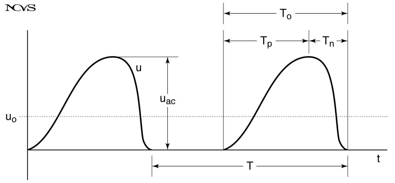 Figure 5.3: A periodic time-domain waveform and its corresponding line spectrum showing discrete harmonics.
Characteristics:
- Components appear only at specific frequencies (fundamental and harmonics)
- Zero amplitude at all other frequencies
- Each line represents a sinusoidal component
- Line heights represent component amplitudes
- Line positions indicate component frequencies
Harmonic Structure:
- Fundamental (f₀): Lowest frequency component, equals repetition rate
- Second harmonic (2f₀): Exactly twice fundamental frequency
- Third harmonic (3f₀): Exactly three times fundamental
- nth harmonic (nf₀): n times fundamental frequency
The harmonic spacing (frequency difference between adjacent harmonics) equals f₀:
Δf = (n+1)f₀ - nf₀ = f₀This spacing provides immediate visual identification of the fundamental frequency.
Continuous Spectra
Aperiodic signals (noise, transients, non-repeating events) produce continuous spectra with energy distributed across a frequency range rather than concentrated at discrete frequencies.
White Noise: Uniform energy distribution across all frequencies; spectrum appears as a flat horizontal line.
Colored Noise: Non-uniform distribution with characteristic spectral shape (pink noise: -3 dB/octave; brown noise: -6 dB/octave).
Transients: Brief, non-repeating events produce spectra with energy distributed according to the temporal envelope.
Speech Consonants: Most consonants (particularly fricatives and stops) have continuous spectra reflecting their aperiodic, noise-like character.
Mixed Spectra
Real voice signals often combine periodic and aperiodic components:
Voiced Sounds: Predominantly periodic (line spectrum) with small amounts of aspiration noise (continuous background).
Breathy Voice: Significant periodic component (harmonics) plus substantial aperiodic component (noise between harmonics).
Rough Voice: Periodic components with amplitude irregularities producing spectral sidebands.
Voiced Fricatives: Simultaneous voicing (harmonics) and friction noise (continuous spectrum).
Components of the Voice Spectrum
Voice spectra reveal multiple layers of information about vocal production.
The Harmonic Series
The most prominent features in voiced sound spectra are the harmonics—spectral lines at integer multiples of f₀.
Fundamental (f₀):
- Lowest frequency component (sometimes labeled H1 or first harmonic)
- Corresponds to vocal fold vibration rate
- Typically 80-300 Hz in speech
- Perceptually corresponds to pitch
Overtones/Harmonics:
- Integer multiples of f₀: 2f₀, 3f₀, 4f₀, …
- Extend to several kilohertz
- Contribute to timbre and voice quality
- Modified by vocal tract resonances
The number of visible harmonics depends on f₀ and analysis bandwidth. Low f₀ produces many harmonics within typical analysis range (0-5 kHz); high f₀ produces fewer.
Example:
- f₀ = 100 Hz: 50 harmonics up to 5000 Hz
- f₀ = 400 Hz: 12-13 harmonics up to 5000 Hz
The Spectral Envelope
Overlaying the fine harmonic structure is the spectral envelope—a smooth curve connecting harmonic peaks representing the overall frequency response.
Determinants:
- Glottal source characteristics: Open quotient, closure pattern, waveform shape
- Vocal tract filtering: Formant resonances and anti-resonances
- Radiation characteristics: +6 dB/octave high-frequency boost at lips
Shape:
- Generally declining amplitude with increasing frequency
- Broad peaks (formants) corresponding to vocal tract resonances
- Valleys (anti-formants) from nasalization or vocal tract zeros
The envelope can be separated from fine structure using:
- Linear predictive coding (LPC): Models vocal tract filter
- Cepstral analysis: Separates source and filter in quefrency domain
- Peak interpolation: Connects harmonic peaks with smooth curve
Spectral Noise
Between and surrounding harmonic lines, spectral noise represents aperiodic energy:
Sources:
- Turbulent airflow (aspiration, breathiness)
- Irregular vocal fold vibration (perturbation)
- Incomplete glottal closure
- Mucosal friction during contact
Quantification:
- Harmonic-to-noise ratio (HNR): Ratio of periodic to aperiodic energy
- Normal phonation: HNR > 15-20 dB
- Pathological phonation: HNR may decrease to <10 dB
Higher spectral noise indicates less efficient phonation and contributes to perceptually rough or breathy voice quality.
Spectral Analysis Parameters
The characteristics of a computed spectrum depend on analysis parameters that involve tradeoffs.
Time Window Length
The duration of signal analyzed determines frequency resolution:
Long Windows (40-50 ms):
- High frequency resolution (good harmonic separation)
- Poor time resolution (averaging across temporal variations)
- Suitable for sustained phonation analysis
- Required for accurate formant measurement
Short Windows (5-10 ms):
- Poor frequency resolution (harmonics may merge)
- High time resolution (captures rapid changes)
- Suitable for dynamic speech analysis
- May not resolve individual harmonics at low f₀
Tradeoff: Time-frequency uncertainty principle limits simultaneous resolution in both domains. The product of time and frequency resolution has a lower bound:
Δt · Δf ≥ 1/(4π)Window Function
Abrupt signal truncation at window edges creates spectral leakage—artificial frequency components due to edge discontinuities.
Window Functions taper the signal smoothly to zero at edges:
Rectangular: No tapering; maximum frequency resolution but worst leakage.
Hamming: Cosine taper; good compromise between resolution and leakage.
Hanning (Hann): Similar to Hamming with slightly different taper.
Blackman-Harris: Extensive tapering; minimal leakage but reduced resolution.
Choice depends on analysis goals: resolution vs. leakage suppression.
FFT Size
The Fast Fourier Transform (FFT) computes the spectrum at discrete frequency points:
Frequency Resolution:
Δf = sampling_rate / FFT_sizeTypical Values:
- Sampling rate: 22050 Hz or 44100 Hz
- FFT size: 512, 1024, 2048, or 4096 points
- Resulting resolution: 10-100 Hz
Tradeoffs:
- Larger FFT → better frequency resolution but requires longer time window
- Smaller FFT → faster computation and better time resolution but coarser frequency resolution
Zero-padding (adding zeros to increase FFT size) interpolates spectrum but does not increase fundamental resolution.
Practical Interpretation of Voice Spectra
Interpreting voice spectra requires understanding what features indicate about vocal function.
Identifying Fundamental Frequency
Method 1—Harmonic Spacing: Measure frequency difference between adjacent harmonics; this equals f₀.
Method 2—Lowest Peak: The lowest frequency harmonic is f₀ (if visible and not filtered out).
Method 3—Cepstral Analysis: Peak in cepstrum (quefrency domain) indicates periodicity, corresponding to f₀.
Challenges:
- Low-frequency energy may be filtered out (high-pass filtering)
- Fundamental may have low amplitude relative to overtones
- Multiple periodicities (diplophonia) produce ambiguous spectra
Formant Identification
Formants appear as broad peaks in the spectral envelope, not as individual harmonics.
Procedure:
- Extract spectral envelope (LPC or smoothing)
- Identify local maxima in envelope
- First peak (lowest frequency) = F1
- Second peak = F2
- Third peak = F3, etc.
Challenges:
- Sparse harmonics (high f₀) may inadequately sample formant peaks
- Adjacent formants may merge if close in frequency
- Nasalization introduces anti-formants (valleys)
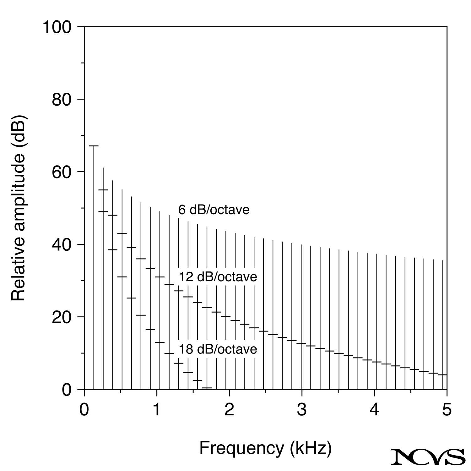 Figure 5.5: Voice spectrum showing harmonic fine structure and formant envelope peaks (F1, F2, F3) representing vocal tract resonances.
Voice Quality Assessment
Different voice qualities produce characteristic spectral patterns:
Normal Modal Voice:
- Clear harmonics extending to 4-5 kHz
- HNR > 15 dB
- Smooth envelope with identifiable formants
- Gradual amplitude decline (~-12 dB/octave)
Breathy Voice:
- Reduced high-frequency harmonic amplitude
- Increased spectral noise (lower HNR)
- Enhanced H1 amplitude relative to H2
- Spectral tilt changes
Pressed/Strained Voice:
- Enhanced high-frequency harmonics
- Steeper spectral slope
- Strong harmonic definition
- Possible subharmonics or biphonation
Rough Voice:
- Reduced HNR
- Spectral irregularities
- Possible subharmonics
- Amplitude modulation sidebands
Clinical Applications
Spectral analysis provides objective measures for clinical voice assessment.
Diagnostic Spectral Features
Harmonic Structure: Clarity and extent of harmonics indicates periodicity of vocal fold vibration.
Spectral Noise Level: Quantified by HNR, indicates glottal closure efficiency and vibration regularity.
Spectral Slope: Changes may indicate altered glottal contact patterns or tissue properties.
Subharmonics: Fractional multiples of f₀ (e.g., f₀/2) indicate period doubling, seen in some pathologies.
Biphonation: Two separate harmonic series indicate independent left-right vocal fold vibration.
Long-Term Average Spectrum (LTAS)
LTAS averages spectra across extended speech samples (30+ seconds):
Advantages:
- Reduces effect of momentary variations
- Characterizes overall spectral balance
- Useful for comparing voice qualities
- Correlates with perceptual dimensions
Applications:
- Vocal training effectiveness
- Professional voice comparison (trained vs. untrained singers)
- Vocal fatigue assessment
- Treatment outcome measurement
Summary
A spectrum represents the frequency-domain description of a signal, showing amplitude or power distribution across frequencies. Based on Fourier’s theorem, any signal can be uniquely decomposed into sinusoidal components, with the spectrum encoding the amplitudes and frequencies of these components. The spectrum is mathematically equivalent to the time-domain representation but often more informative for acoustic analysis.
Periodic signals produce line spectra with discrete harmonics at integer multiples of the fundamental frequency, while aperiodic signals produce continuous spectra. Voice spectra typically combine both types, showing harmonics (from periodic vocal fold vibration) plus noise components (from aspiration and turbulence). The spectral envelope overlaying the harmonic fine structure reveals formant patterns reflecting vocal tract resonances.
Practical spectral analysis involves tradeoffs between time and frequency resolution, managed through window length, window function, and FFT size selection. Interpretation of voice spectra enables identification of fundamental frequency, formant frequencies, and voice quality characteristics. Clinical applications include objective measurement of harmonic structure, noise levels, and spectral balance for diagnosis and treatment monitoring.
Key Takeaways
- ✅ A spectrum shows amplitude or power distribution across frequencies, equivalent to time-domain representation
- ✅ Fourier’s theorem enables decomposition of any signal into sinusoidal components
- ✅ Periodic signals produce line spectra with harmonics at integer multiples of f₀
- ✅ Aperiodic signals produce continuous spectra with distributed energy
- ✅ Voice spectra combine harmonic fine structure (from vocal fold vibration) and spectral envelope (from vocal tract filtering)
- ✅ Spectral analysis parameters involve tradeoffs between time and frequency resolution
- ✅ Clinical spectral measures include HNR, spectral slope, and LTAS for voice quality assessment
Related Topics
- Frequency Spectra & Spectral Slope
- The Spectral Slope
- The Glottal Source Function
- Periodicity
- Simple Harmonic Motion
Further Reading
- Titze, I. R. (2000). Principles of Voice Production (2nd ed.). Iowa City: National Center for Voice and Speech.
- Fant, G. (1960). Acoustic Theory of Speech Production. The Hague: Mouton.
- Stevens, K. N. (1998). Acoustic Phonetics. Cambridge, MA: MIT Press.
- Baken, R. J., & Orlikoff, R. F. (2000). Clinical Measurement of Speech and Voice (2nd ed.). San Diego: Singular Publishing Group.
- Oppenheim, A. V., & Schafer, R. W. (2009). Discrete-Time Signal Processing (3rd ed.). Upper Saddle River, NJ: Prentice Hall.