Fourier Transformations

Fourier transformation (named after French mathematician Joseph Fourier, 1768-1830) is the process of transforming events in time to frequencies. The time course of events is usually called a waveform or signal, and the collection of frequencies is called a spectrum. Basically, we ask: what collection of sinusoids can be added together to represent the waveform in its full detail?

The Gaussian Waveform Example

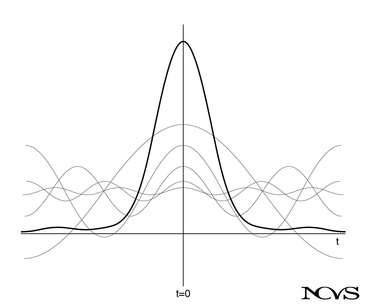
Figure 6.14: Construction of a bell-shaped (Gaussian) waveform from a collection of sinusoids. In theory, it requires an infinite number of sinusoids with frequencies spaced infinitesimally close.

As a first example, consider how a bell-shaped (Gaussian) waveform is constructed from a collection of sinusoids. In theory, there should be an infinite number of sinusoids spaced infinitesimally close in frequency.

Properties of the Gaussian Signal

At t = 0, the sinusoids add together in phase, giving a peak in the waveform. On either side of the peak, the sinusoids do not add in phase as time moves to either plus infinity or minus infinity. At no time does another peak occur.

We say that although the waveform is continuous, it is:

• Localized near t = 0

• Non-periodic (has no repetition)

• Contains no fundamental frequency, even though an infinite number of frequencies are present

The Gaussian Transform Pair

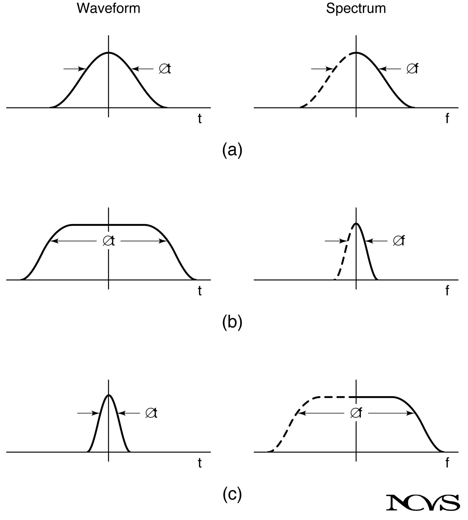
Figure 6.15: Waveforms (left) and corresponding spectra (right): (a) a bell-shaped (Gaussian) waveform, (b) broadening the waveform duration, and (c) narrowing the waveform duration.

This bell-shaped curve is special because it has a mirror image as its spectrum. The distribution of frequencies (right side) is the same as the distribution of events in time (left side). Each frequency is represented by a point on the curve, with the height representing the amplitude of the respective sinusoid, but the points are so closely spaced that they make a continuous spectrum.

Mathematical Note on Negative Frequencies

Negative frequencies (shown with dashed lines) are also obtained mathematically by Fourier transformation, but they have no physical interpretation. They arise from the mathematical representation using complex exponentials and can be ignored for practical purposes.

The Inverse Time-Frequency Relationship

A fundamental principle emerges from the Gaussian example:

If we broaden the waveform (Figure 6.15b):

• Duration in time increases

• Spectrum narrows

• Fewer high frequencies are needed

• Bandwidth decreases

If we narrow the waveform (Figure 6.15c):

• Duration in time decreases

• Spectrum broadens

• More high frequencies are needed

• Bandwidth increases

Mathematical Expression

This inverse time-frequency relation can be expressed as:

Δt ∝ 1/Δf

where:

• Δt = duration of events in time

• Δf = frequency bandwidth of the spectrum

Interpretation: A smaller duration of events requires a greater frequency bandwidth, and a greater duration of events requires a smaller frequency bandwidth.

Extreme Cases

The Sharp Pulse (Impulse)

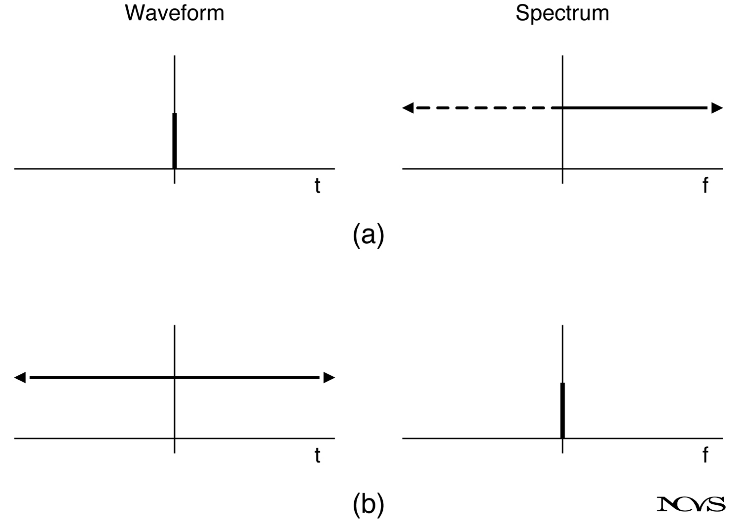
Figure 6.16: (a) A sharp pulse and its spectrum and (b) a constant (in time) and its spectrum.

When the duration of events shrinks to zero (a sharp pulse or impulse):

• Waveform: Infinitely narrow spike

• Spectrum: Infinite bandwidth (all frequencies present with equal amplitude)

• Physical interpretation: A click or impulse contains all frequencies

The Constant Signal

In the opposite extreme, when event duration is infinite (a constant for all time):

• Waveform: Horizontal line (no variation)

• Spectrum: Zero bandwidth (only DC, no frequencies)

• Physical interpretation: No acoustic signal, just steady pressure

Non-Periodic Signals

Random Pulses (Band-Limited Noise)

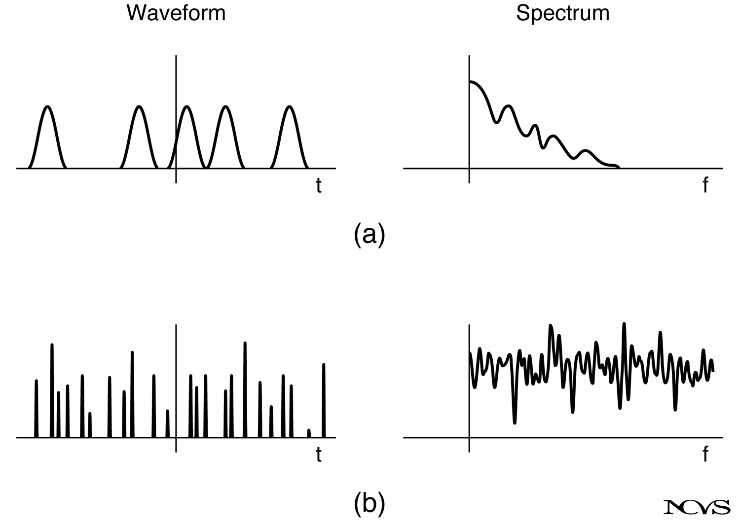
Figure 6.17: (a) Waveform and spectrum for broad pulses repeated at random intervals and (b) random sharp pulses (noise) and spectrum.

Consider a series of rounded pulses that are non-periodic. Individual pulses are similar, but the interpulse interval is random, suggesting that no portion of the waveform is ever repeated precisely.

Characteristics:

• Overall bandwidth determined by pulse shape

• Random hills and valleys in spectrum

• No discrete frequency lines

• Called band-limited noise

White Noise

When each pulse becomes very sharp:

• Spectrum includes all frequencies

• Random hills and valleys remain

• Overall bandwidth is infinite

• Called white noise (analogy to white light containing all optical frequencies)

By analogy, band-limited noise is called colored noise because colors appear when optical frequencies are removed from white light.

Periodic Signals

Repeated Pulses (Glottal Flow)

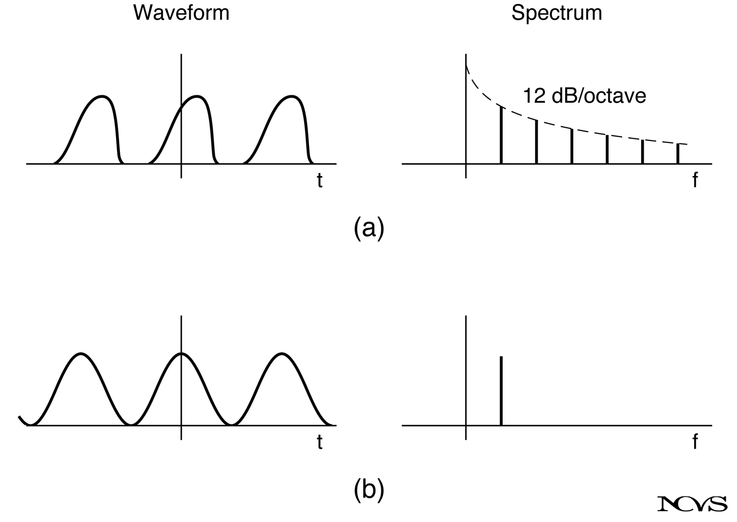
Figure 6.18: (a) Waveform and spectrum for pulses repeated at periodic intervals, such as glottal flow pulses, and (b) a sinusoid and its spectrum.

When repeated pulses are periodic (equally spaced in time):

Waveform characteristics:

• Regular repetition rate

• Constant interpulse interval

• Period T = 1/F₀

Spectrum characteristics:

• Regularly spaced lines

• First line at fundamental frequency F₀

• All other lines are harmonics (integer multiples of F₀)

• Prolonged deep valleys where there is no amplitude

• Overall bandwidth quantified by spectral slope (e.g., 12 dB/octave)

This is exactly the spectrum of the glottal airflow waveform discussed in Chapter 5.

The Pure Sinusoid

The simplest periodic signal is a sinusoid:

Waveform:

• Single frequency

• Extends from minus infinity to plus infinity in time

• Smoothly connected repetitive pattern

Spectrum:

• Single line

• One frequency only

• Trivial but important limiting case

Practical Implications

For Voice Analysis

The inverse time-frequency relationship has important implications:

1. Short analysis windows (brief samples):

  - Broad frequency bands

  - Poor frequency resolution

  - Good time resolution

  - Suitable for tracking rapid changes

2. Long analysis windows (extended samples):

  - Narrow frequency bands

  - Good frequency resolution

  - Poor time resolution

  - Suitable for steady-state analysis

For Understanding Voice Signals

Different voice signals have characteristic spectra:

• Vowels (periodic glottal pulses): Line spectrum with harmonic structure

• Voiced consonants: Similar to vowels but may have additional noise

• Voiceless consonants: Continuous spectrum (noise-like)

• Transitions: Time-varying spectra requiring time-frequency analysis

Summary

Fourier transformation is the mathematical process of decomposing time-domain signals into their frequency components. The fundamental principle is an inverse relationship between time duration and frequency bandwidth: shorter events require broader frequency ranges, and longer events require narrower frequency ranges. Periodic signals produce line spectra with discrete frequencies, while non-periodic signals produce continuous spectra. The Gaussian waveform is unique in having a Gaussian spectrum, making it a perfect example of the time-frequency relationship.

Key Takeaways

• ✅ Fourier transformation decomposes waveforms into collections of sinusoids

• ✅ There is an inverse relationship between time duration and frequency bandwidth (Δt ∝ 1/Δf)

• ✅ Sharp pulses require infinite bandwidth; constants require zero bandwidth

• ✅ Periodic signals produce line spectra with harmonics

• ✅ Non-periodic signals produce continuous spectra

• ✅ The Gaussian waveform has a Gaussian spectrum (mirror image)

Related Topics

• Filters and Filtering

• The Sound Spectrograph

• Glottal Flow Spectrum

• Formant Bandwidth

Further Reading

1. Poularikas, A., & Seely, S. (1985). Signals and systems. Boston: PWS-Kent Publishing.

2. Pickett, J. M. (1980). The sounds of speech communication. Baltimore: University Park Press.

3. Borden, G. J., & Harris, K. S. (1980). Speech science primer. Baltimore: Williams & Wilkins.